So, the inspiration for this blogpost came after coming across this interesting graph made in R:
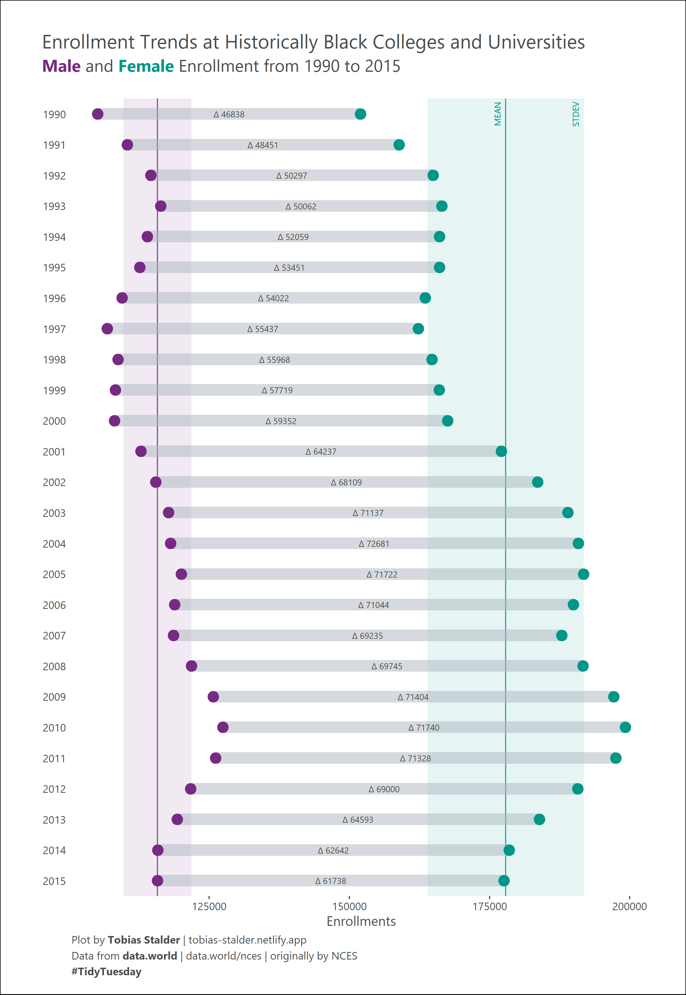
What caught my attention were two things:
- This was a dumbbell plot displaying time series vertically. It’s a bit strange, since I’m accustomed to visualizing time series horizontally.
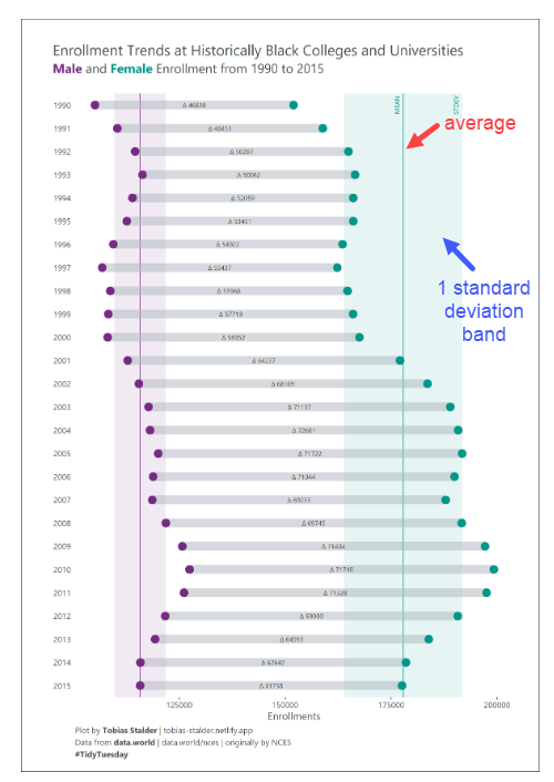
- The two series displaying the total enrollments by year by genre (Female and Male) had each, an average line (red arrow below) along with a 1 standard deviation band +/- from the average (blue arrow). This is interesting because it adds context and more perspective to the graph.
After finishing reading how it was created in R, I started to think how we can make this chart in mighty Excel. To be honest, on my own I struggled a bit. I tried many approaches, and nothing seemed to work until I got to meet Mr. Bolaji Olatunde through a Zoom call.

Bolaji showed me an interesting solution with stacked bars yet, when plotted, the widths of standard deviation bands were not fully precise to their corresponding axis. After two hours or so of going back and forth with other alternatives, we came up with the idea of using error bars to display the standard deviation bands. We tested it and it worked! Below is the solution that we produced:
This was an amazing Zoom call because I got to collaborate with somebody else (who I met for the first time) to make an interesting graph in Excel. To Bolaji, thank you! Dear reader, make sure you check out his work with Power BI on LinkedIn, it’s quite impressive.
Now, let’s proceed to make a dumbbell plot in Excel with average reference lines and 1-standard-deviation-bands along with adding Dynamic Arrays to make it: interactive. 🔥
Note: I’m a visual person so, after every written step I will demonstrate the same with a small video clip.
Step 1: Margins are sacrosanct.
We add one column to the left and one row above the range of values that we will be working with. Select the entire range of data with CTRL + * (asterisk) and then convert it into an Excel table with CTRL + T. In the Create Table dialog box, make sure “My table has headers” is checked. Clik OK. Go to the Table Design tab and rename this table from Table1 to _01_data, then switch the Table Style to White, Table Style Light 4.
Step 2: We add the following formula below on cell I2:
= UNIQUE( _01_data[[#All],[channel]] )
On this spilled array we use the UNIQUE function to obtain the unique items (including the header) from column channel of table _01_data. In the Name manager, we map this spilled array with the following name: _02_channels and then, in the Refers to box: add the # at the end of the absolute cell reference. Click OK.
Step 3: let’s create a pivot table from this named spilled array: _02_channels
Yes, this is awesome: you can link a “named spilled array” to a pivot table. In other words, you can have a spilled array result as the source of a pivot table, as long as the spilled arrays have headers on the first row and the spilled array is named or mapped in the Name Manager of the workbook. Another benefit of linking a “named spilled array” to a pivot table is that if the data grows in the Excel table, you will only have to update the whole workbook to grab the latest items in their respective columns. For refreshing the whole workbook, just go to the Data tab and then click on Refresh All.
Now, to link a named spilled array to a Pivot Table, click on Insert Pivot Table, then in the PivotTable from table or range dialog box, on section Table/Range, press F3 or Fn + F3 (on laptop) and from the Paste Name dialog box, click on _02_channels, then click OK. Now, click on Existing Worksheet and change the location to be cell K2 then click OK.
Almost done, let’s proceed with the following formatting changes, right click on the pivot table, and go to Pivot table options, then:
- Rename this pivot table from PivotTable1 to pt_channels (pt = pivot table)
- Uncheck this annoying option: Autofit column widths on update. Click OK.
- On the contextual PivotTable Design tab, go to section Report Layout, and switch the layout from Show in compact form to Show in Tabular form.
- On section PivotTable Style Options, turn off Row Headers.
- On the section of PivotTable styles switch it to White, Pivot Table Style Light 1.
- Add the channel field to the Rows quadrant in the PivotTable Fields pane.
- Remove the grand total from the pivot table.
- Let’s add the slicer: Channels and rename it in the name manager to _03_channels_slicer. Clik OK.
- Now, click on the items of the slicer and check how the pivot table changes dynamically with one click.
Step 4: let’s format the aesthetic of this slicer and following ones.
- Click on the added slicer. Then go to the contextual tab: Slicer.
- Under section Slicer Styles, switch it to White, Slicer Style Light 3.
- Then right click on this style and go to Duplicate.
- On the Modify Slicer Style dialog box, change the name to “custom”.
- Then click on Whole Slicer and then click the Format button.
- On the Font tab, select the font type: Arial, then size 8.
- Then go to the Border tab, click None on the Presets section. Click OK.
- Now click on Header and then click on the Format button. Repeat step 7.
- Now on the Modify Slicer Style dialog box, in all the items below Header, you will repeat step 7.
- Once done, and in the Modify Slicer Style dialog box, click OK.
- Finally, switch the style of slicer to the new one.
Now it seems like a lot to do, but you won’t need to build a macro, because you can copy-and-paste this slicer to another workbook and this custom setting will transport as is. : ) Let’s continue.
Step 5: we add the following formula below on cell M2.
= UNIQUE( _01_data[[#All],[category]:[subcategory]] )
Like the spilled array formulated in Step 2 but this time with two columns. No need to sort this array because each column will be individually sorted once displayed on their respective pivot tables. Finally, we map this spilled array formula in the name manager like we did in step 2 with _04_categories.
Step 6: It’s like step 3 but we need to create two pivot tables and two slicers with a small difference on these last two.
Let’s continue Friday Oct 7th.